Team Name: DocileDolphins

Cleophas Kalekem, Ted McNulty, Chong Swee, Jiaxuan (Amy) Wu

Software Systems

2/27/2017

Project 1 Final Report

Big Idea/Abstract

Our goal for this project was to demonstrate the properties of the Brachistochrone Curve using our own physics engine. The Brachistochrone Curve demonstrates two properties. First, a ball at the top of the slope will reach the bottom of the slope faster than any other type of curve or ramp. Second, the amount of time the ball takes to reach the bottom of the slope is constant, regardless of where the ball starts, whether it be at the very top, or a few inches from where the ball would naturally land.

These two properties arise because of the curve having such fine and specific detail. The more details an object has, the more triangles we need to use to represent it. This creates a problem because collision detection for objects constructed with triangles is computationally expensive. In a perfect simulation, the triangles which construct the curve would be infinitely small, however this is not realistic. We were left with a tradeoff between decreasing the number of triangles and sacrificing the fine detail that is necessary for the curve. Later research suggested that even the complex polygon collision detection algorithm we were considering using (Separating Axis Theorem) isn’t reliable when detecting concave structures, such as curves.

Regardless of the difficulties with the curve, we wanted to demonstrate our personal physics engine, so we instead tried to focus on a ball realistically bouncing off of a surface, regardless the angle the ball was thrown or the angle of the surface.

Background

Our physics engine is a simple version of one that might be used in a simulation or a video game, with the help of rendering software like OpenGL, which we used. The basic idea of OpenGL and a physics engine are straight forward; you can create objects defined in classes or structures. For example take a look at Gameobject.h:

class Gameobject{

	//Everything in here is public
	public:

	//Constructor
	Gameobject();

	//Deconstructor
	~Gameobject();

	//Draw the object on the screen
	void draw();

	//Print Diagnostic reports
	void print();

	//Apply gravity and collision detection
	void apply(Physics p);

	//Position represented with a array of floats
	void setP(float* positon);
	void setP(float x, float y, float z);
	float* getP();

	//Acceleration represented with a vector
	void setV(float* velocity);
	Vectorobject getV();

	//Acceleration represented with a vector
	void setA(float* accelation);
	Vectorobject getA();

	float gravity;

	//Everything here can only be used within the class
	protected:


	float p[3];	//Position represented with 3 coordinates

	Vectorobject v;	//Velocity

	Vectorobject a; //Acceleration
};

This is our parent class for all objects and provides us a good example for understanding OpenGL and physics engines. Everything we do in OpenGL is to model the real world, because that’s the actual goal. Therefore, like in the real world and real physics, every object has some position in space:

float p[3];	//position represented with 3 coordinates

Every object has a velocity in all 3 directions (although it may be 0):

Vectorobject v; //Velocity

And every object is also accelerating in all 3 directions (again, might be 0):

Vectorobject a; //Acceleration

In a more complex engine, there will probably even be fields to store the mass of the object, or the resistance of the material the object is made of. Nonetheless, with position, velocity, and acceleration we can accurately model simple projectile motion with equations like

v.final = v.initial + acceleration*delta.time

So with the limited information the objects have they can just use the basic kinematic equations necessary to model real physics. But how does it show the simulation on the screen? That’s where OpenGL comes in.

As previously alluded to, OpenGL is a graphics library that makes it rather simple to create a new window and draw objects in, and is very efficient in doing so. The basic premise of how OpenGL works is again, modeled after real life. We have a camera (sometimes referred to as eye) “object”, light objects, and all the objects you want to draw. All these things have positions on an x,y,z plane and the camera and lights also store the point they are facing. When the code is run, it simulates light (in the form of rays) bouncing away from the camera lens, each ray corresponding to a pixel in the window. When each ray hits something (or doesn’t), it knows what it hits (or doesn’t) and therefore knows what color to assign to the pixel (still does).

This process is actually being done every frame, or about every 250ms. The magic comes from this little command:

   glutIdleFunc(display);

Which says, whenever the program is idle and is ready to exit, run the function display. Display is where we are adding our objects to draw to the buffer, so every single frame it does all the computation completely over again. You can take advantage of this by using the structures or classes suggested above. If we simplify the drawing function down to sphere.draw(), for say a sphere, we could modify the position of the sphere in another function, and the next time sphere is drawn, it would appear to move.

There are essentially 2 ways to represent objects in OpenGL, you can have a sphere or construct a more complex object by creating triangle faces which share edges. For example a cube would be made of 12 triangles (because it has 6 sides and 2 triangles are need to make a square), and every edge of a triangle would be shared with another triangle. A sphere however, can be done simply by defining the radius, since collision detection is quite simple with just a sphere and a ray, and constructing a sphere with triangles would be futile.

However, we used the GL Utility Toolkit to help with some of the dirty work regarding creating a cube with triangles and creating the sphere. GLUT also provided us with some nice functions to easily create the window.

Implementation

We were able to create a physics engine which accurately models the physics of a bouncing ball, both on a flat plane and an angled plane. This also consists of an accurate gravity simulation where each item affected by gravity will slowly approach free-fall under gravity (as opposed to just having the y-velocity of each set to -9.8 manually). Furthermore, the engine also needed to have accurate collision detection between a plane (represented as a scaled cube for our purposes) and a sphere. Lastly, we were able to create this engine strictly with formulas related to projectile motion and similar fields of physics (formulas such as the dot product and cross product of vectors, or calculating position, velocity, and acceleration given a difference in time).

Given our problem space, there is really only one major decision for us to make regarding the design implementation of this project (since a lot of the implementation is out of ours hands, being it’s physics), which is choosing an algorithm for collision detection. There are 3 main ways we found to create collision detection:

1. Bounding boxes

   Bounding boxes, takes every object and it frames a box around it, as small as possible, this box acts as a hitbox for the object, and can be effective for many shapes, but for something like a sphere, it loses its effectiveness. If an object approaches the sphere within the box from the direction of one of the corners of the box, the collision detection will report a collision sooner than it should.

2. Bounding spheres

   So bounding boxes are effective for cube-like shapes, but we are dealing mostly with a sphere so we also considered bounding spheres. This takes the same concept, but instead of surrounding the object with a box for a hitbox, we surround it with a sphere. This is actually easier to calculate than a bounding box collision since all we have to do is make sure the distance between two objects are less than their radii. Again, this algorithm falls short for non-sphere objects.

3. Separating-Axis theorem

   Finally we considered the Separating Axis-Theorem, which is a professional algorithm which is specifically designed for collision detection between complex polygons, instead of simple cubes or spheres. As you might suspect, because this algorithm can handle such complex shapes it sacrifices a lot of run time (as it needs to compare every face to every other face, instead of just every object to every other object). Not only would this algorithm slow our simulation down significantly, but it also can only handle convex polygons, not concave polygons (like a slope). With these facts, we decided Separating Axis-Theorem would not be helpful.

We compromised by implementing a cross between bounding boxes and bounding spheres by implementing bounding boxes for the cube-like objects and bounding spheres for sphere-like object. We believe this was the correct choice as we could set up the simulation with just spheres and cubes, and it gave us a chance to write our own Cube/Sphere collision detection algorithm.

//From Sphereobject::apply(Physics p);
//
//Recalculates position, velocity, and acceleration for a given sphereobject and time since last update
//This is only the section that recalculates velocity
//
//If there is no intersection
if(intersects==0){
		//Velocity equals acceleration times the difference in time
		temp_values2[i]=diff*temp_acceleration[i] + temp_velocity[i];
}
//If there was intersection
else{
	//make an int for looping
	int j;

	//Calculate the sum of the normal vector of the plane you are hitting
	normal_sum= plane.getN().get()[0] + plane.getN().get()[1]+ plane.getN().get()[2];
	//Calculate the sum of the velocity vector (absolute value to ignore direction)
	velocity_sum= fabs(temp_velocity[0])+fabs(temp_velocity[1])+fabs(temp_velocity[2]);

	//Allocate for energy lost in collision
	velocity_sum= velocity_sum*0.6;

	//Divide the total momentum by the sum of the vector (how many ways do we need to divide the energy up)
	velocity_sum= velocity_sum/normal_sum;

	//For each axis
	for(j=0;j<3;j++){

		//Given the plane's normal at i is NOT 0
		if(plane.getN().get()[i]!=0){

			//Add velocity at i based on the momentum times the normal of the plane at i
			temp_values2[i]=velocity_sum*plane.getN().get()[i];
		}
	}
}

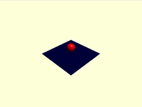
Results

Below you can see two video recordings of our physics engine at work. The first is a ball that falls onto a flat plane and bounces until it comes to a resting position. The second is a ball bouncing down a 45 degree slope to illustrate the engine’s ability to handle any angle of slope or of the ball’s velocity.